74
Tecnología y Ciencias del Agua
, vol. VIII, núm. 2, marzo-abril de 2017, pp. 71-76
Zheng & Yu,
Improvement of vertical “scatter degree” method and its application in evaluating water environmental carrying capacity
•
ISSN 2007-2422
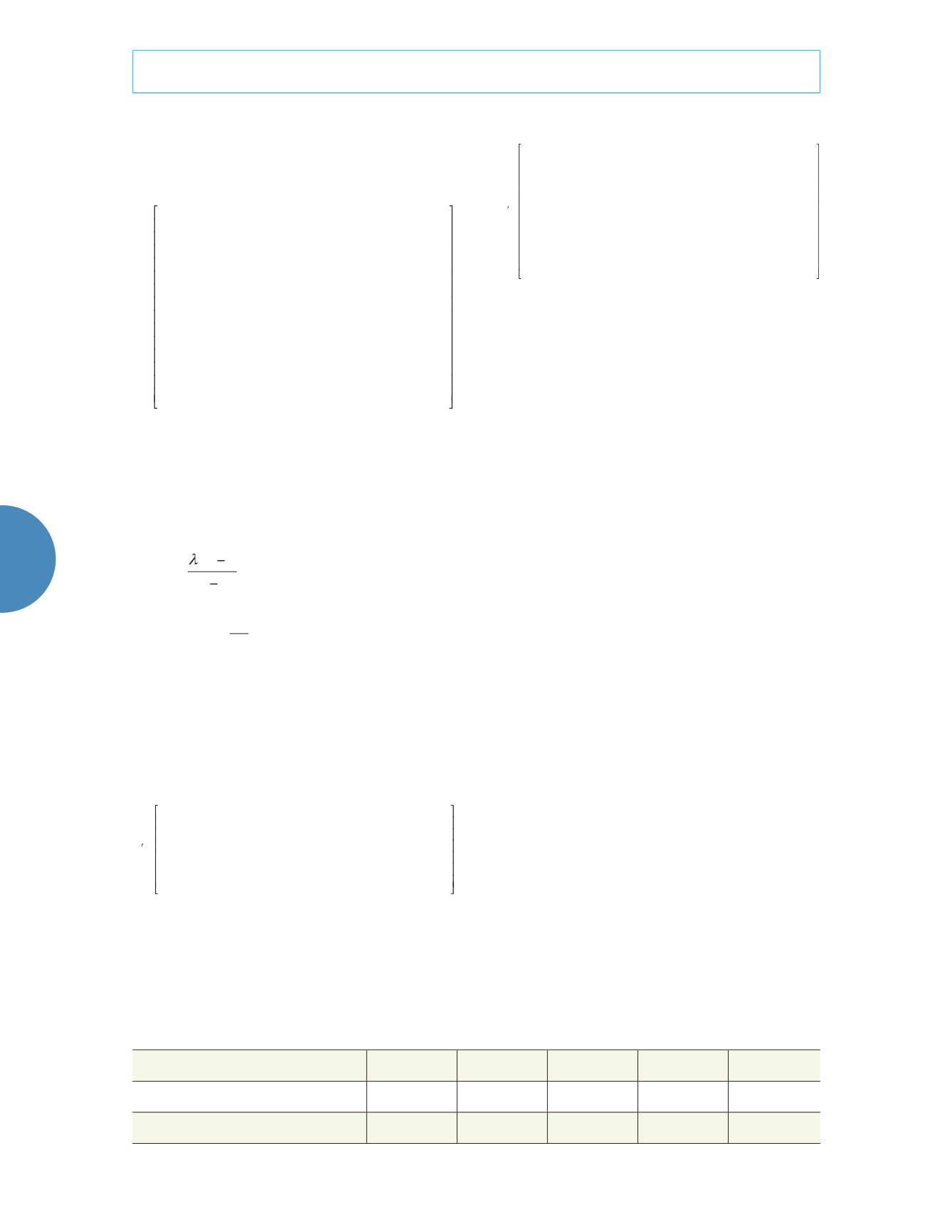
reference to the literature. Then, matrix B is
acquired as follows:
B
=
X
1
X
2
X
3
X
4
X
5
X
6
X
7
X
8
X
9
X
1
1.00 1.00 0.33 0.25 0.33 0.33 0.50 0.50 0.25
X
2
1.00 1.00 0.33 0.25 0.33 0.33 0.50 0.50 0.25
X
3
3.00 3.00 1.00 0.50 1.00 1.00 2.00 2.00 0.50
X
4
4.00 4.00 2.00 1.00 2.00 2.00 3.00 3.00 1.00
X
5
3.00 3.00 1.00 2.00 1.00 1.00 2.00 2.00 0.50
X
6
3.00 3.00 1.00 0.50 1.00 1.00 2.00 2.00 0.50
X
7
2.00 2.00 0.50 0.33 0.50 0.50 1.00 1.00 3.00
X
8
2.00 2.00 0.50 0.33 0.50 0.50 1.00 1.00 3.00
X
9
4.00 4.00 2.00 1.00 2.00 2.00 0.33 0.33 1.00
Then, the weight of the indicator is obtained
by using MATLAB:
l
max
= 9.886,
r
= (0.043, 0.043,
0.127, 0.217, 0.127, 0.127, 0.092, 0.092, 0.133)
T
.
3. Consistency check: 1) consistency index:
max
1
n
CI
n
=
, where n is the number of
indicators, and
CI
= 0.11075; 2) consistency
ratio:
CI
CR RI
=
, where
RI
is the mean random
consistency index, and when
n
= 9,
RI
= 1.46.
So,
CR
= 0.07586 < 0.10, and the judgment
matrix is consistent.
The WECC of AHP-Vertical “scatter degree”.
The matrix
X
’ is acquired using Eq. (7).
X
=
0.430 0.000 0.000 0.000 0.997 0.000 0.765 0.401 0.803
0.000 0.059 0.325 0.635 1.270 0.314 0.920 0.000 1.330
0.193 0.155 0.745 1.515 1.246 0.328 0.000 0.806 0.437
0.030 0.344 1.113 1.711 0.303 1.082 0.788 0.920 0.000
0.237 0.430 1.270 2.170 0.000 1.270 0.749 0.835 0.039
A symmetric matrix
H
’ is derived from the
formula:
H
'
=
X
'
T
X
'
H
=
0.2792 0.1421 0.4780 0.8576 0.6779 0.3965 0.5303 0.5533 0.4389
0.1421 0.3309 1.0641 1.7944 0.3724 0.9879 0.6479 0.8007 0.1631
0.4780 1.0641 3.5134 5.9959 1.6781 3.1638 2.1279 2.6855 0.8069
0.8576 1.7944 5.9959 10.3342 3.2128 5.3027 3.5588 4.6069 1.5915
0.6779 0.3724 1.6781 3.2128 4.2517 1.1347 2.1701 1.6833 3.0346
0.3965 0.9879 3.1638 5.3027 1.1347 2.9897 2.0935 2.3199 0.6104
0.5303 0.6479 2.1279 3.5588 2.1701 2.0935 2.6150 1.6580 1.8678
0.5533 0.8007 2.6855 4.6069 1.6833 2.1399 1.6580 2.3544 0.7072
0.4389 0.1631 0.8069 1.5919 3.0346 0.6104 1.8678 0.7072 2.6068
The maximal eigenvalue and eigenvector
of matrix
H
’ is calculated using MATLAB:
l
max
’(
H
’) = 22.22,
w
’(
H
’) = (0.0260, 0.0442, 0.1490,
0.2570, 0.1046, 0.1322, 0.1066, 0.1177, 0.0627)
T
.
The values of WECC in the years of 2005
and 2009 were calculated by putting
x
j
(
t
k
) and
w
j
’ into Eq. (2). The results are shown in table 1.
From the table and figures, it is clear that the
results of the evaluation are basically consistent.
Conclusions
By comparing the results of the two methods,
the conclusions are as follows: (1) The trend of
the two methods’ calculation of the WECC is
the same; namely, the WECC is enhanced. This
enhancement in WECC is closely related to the
strengthening of the environmental governance,
upgrading of production equipment, and the
improvement of water-saving and environ-
mental awareness; (2) As the two groups of
data were calculated and compared, the WECC
of 2005 was found to be 0.3677 or 0.2947 with
the two models, respectively. From this data, it
shows that the WECC of 2006 increased 11.59%
and 93.45% relative to the WECC of 2005 by ver-
tical “scatter degree” method and AHP-vertical
“scatter degree” method. Based on the original
data of the reference, there were eight indica-
tors’ data of 2006 higher than them of 2005, and
their increasing rates were mostly greater than
Table 1. The results of WECC by two different methods.
Year
2005
2006
2007
2008
2009
Vertical “scatter degree” method
0.3677
0.4103
0.5108
0.6925
0.7712
AHP-Vertical “scatter degree” method
0.2947
0.5701
0.8083
0.9886
1.1206


